

OpenVINO Blog

OpenVINO GenAI Supports GGUF Models
Authors: Fiona Zhao, Xiake Sun, Su Yang, Tianmeng Chen
1. Introduction:
This blog introduces the technical details of OpenVINO GenAI GGUF Reader and provides the Python and C++ implementations of OpenVINO GenAI pipeline that loads GGUF models, create OpenVINO graphs, and run GPU inference on-the-fly. To help customers integrate their existing llama.cpp-based LLM applications with OpenVINO inference, OpenVINO provides two approaches for GGUF support currently. Users can access the preview feature of the online GGUF Reader starting from the OpenVINO GenAI 2025.2 release.
GGUF (GGML Universal File Format) is the model format used by llama.cpp, a C/C++-based LLM inference framework. Models are typically trained in PyTorch, then converted and quantized into GGUF for use with llama.cpp.
The offline GGUF-to-OpenVINO approach converts and dequantizes the GGUF file into an FP16 PyTorch model. Subsequently, you can convert the PyTorch model into OpenVINO INT4 model via optimum-cli. The advantage of offline conversion is that it generates a unified OV model, which can be deployed with the C++/Python GenAI pipeline on different Intel platforms (including NPU). The drawback is the additional storage and processing overhead for PyTorch model dequantization and OV NNCF quantization. In this blog, we will focus on the second approach: Online GGUF Reader.
Key Features:
- - One-Step Loading: Directly read, unpack, and convert GGUF-compressed tensors to OpenVINO format in a single API call.
- - On-The-Fly Graph Creation: No intermediate PyTorch model and offline conversion with optimum-cli.
- - Integrated Dequantization: Handle dequantization during inference, eliminating extra storage and preprocessing steps.
- - Simplified Dependency Management: Zero PyTorch/Optimum dependencies.
2. Model library:
Validated model scope and platforms:
*Q8_0 GGUF is limited to MTL GPU, while FP16 GGUF works across MTL, LNL, and ARL GPUs.
Qwen/Qwen2.5-0.5B-Instruct-GGUF is a corner case, because Qwen2.5-0.5B-Q4KM contains a rarely used and unsupported q5_0 tensor.
In the OpenVINO GenAI 2025.2 release, the GGUF Reader does not support Qwen3 GGUF models. Support for Qwen3 GGUF is currently a work in progress (WIP) and will be added in a future update.
Our validation focuses on the widely used quantization type Q4_K_M.
Below is the list of Q4_K_M GGUF models validated on both CPU and GPU platforms (MTL, LNL, and ARL).
3. Usage:
OpenVINO GenAI provides implicit GGUF support based on the file extension, rather than through a separate GenAI GGUF sample. Users can create an LLMPipeline directly from a .gguf file.
Python Usage:
We provide a single Python script that downloads the GGUF model and runs it with the GenAI pipeline on-the-fly.
https://github.com/sammysun0711/openvino_aigc_samples/tree/gguf_ov_genai/GGUF-OV
C++ Usage:
Referring to this blog, How to Build OpenVINO™ GenAI APP in C++, build the OpenVINO GenAI pipeline using the OpenVINO Archive.
1. Download the latest OpenVINO Archive and Install dependencies.
Here, we use Windows to run qwen2.5-1.5b-instruct-q4_k_m.gguf as an example.
Once downloaded, unzip the downloaded file and extract the contents to <your_path>\openvino_genai_windows_2025.2.0.0.dev20250515_x86_64
2. Build OpenVINO GenAI example:
Open a command prompt and run setupvars.bat from the extracted OpenVINO GenAI folder.
<your_path>\openvino_genai_windows_2025.2.0.0.dev20250515_x86_64\setupvars.bat
Modify the file samples/cpp/text_generation/greedy_causal_lm.cpp to add GGUF file and OV tokenizer as input, and to enable GPU inference.
In the same command window, after the OpenVINO environment is initialized, navigate to the folder samples/cpp/, and run build_samples_msvc.bat.
Once the build process is complete, you will find the greedy_causal_lm.exe file in the path indicated in the build output.
3. Download LLM and Tokenizers
Download OpenVINO Tokenizers for Qwen2.5 models. (All Qwen2.5 parameter variants can share the same OpenVINO tokenizer IRs.)
Copy the above code into Notepad and save it as download_file.bat (ensure the file extension is .bat, not .txt). Run it by typing download_file.bat in the Command Prompt.
Or convert OpenVINO Tokenizers for the latest or other llama-based models (optional)
4. Run GGUF
4. Limitations
1.Tokenizer Conversion
In GenAI 2025.2, online conversion of GGUF tokenizers to OpenVINO (OV) format is not yet supported. This capability is a work in progress and is planned for inclusion in a future release.
As a workaround, we can download the OpenVINO tokenizer or perform offline conversion for use with the C++ pipeline, as shown in the usage section.
2.GPU INT8 kernel Group-size issues for q6_k and q8_0
Both Q4_0 model (last layer) and Q4KM GGUF model have q6_k GGUF tensor. Q8_0 GGUF has q8_0.
These GGUF-converted OpenVINO IR models work with CPU inference but fail on LNL and ARL GPUs.
OV INT8 is channel-wise by default, but q6_k’s group-size is 16, while q8_0’s group-size is 32. Currently INT8 dequantization has oneDNN issue.
To support Q4_0 and Q4KM, workaround for q6_k is to convert q6_k to f16 instead of q6_k-to-int8. This has an impact on Q4KM performance (most tensors of Q4KM are q4_k). It is recommended to use Q4_0 GGUF for better performance.
* Q8_0 has a oneDNN accuracy issue on LNL and ARL GPUs, and currently, no workaround is available for these platforms.
5. Technical Details
OpenVINO GenAI GGUF Reader: Simplify LLM deployment with direct GGUF model loading and optimized inference. No PyTorch dependencies, no additional conversions with intermediate PyTorch model, just high-performance inference out of the box.
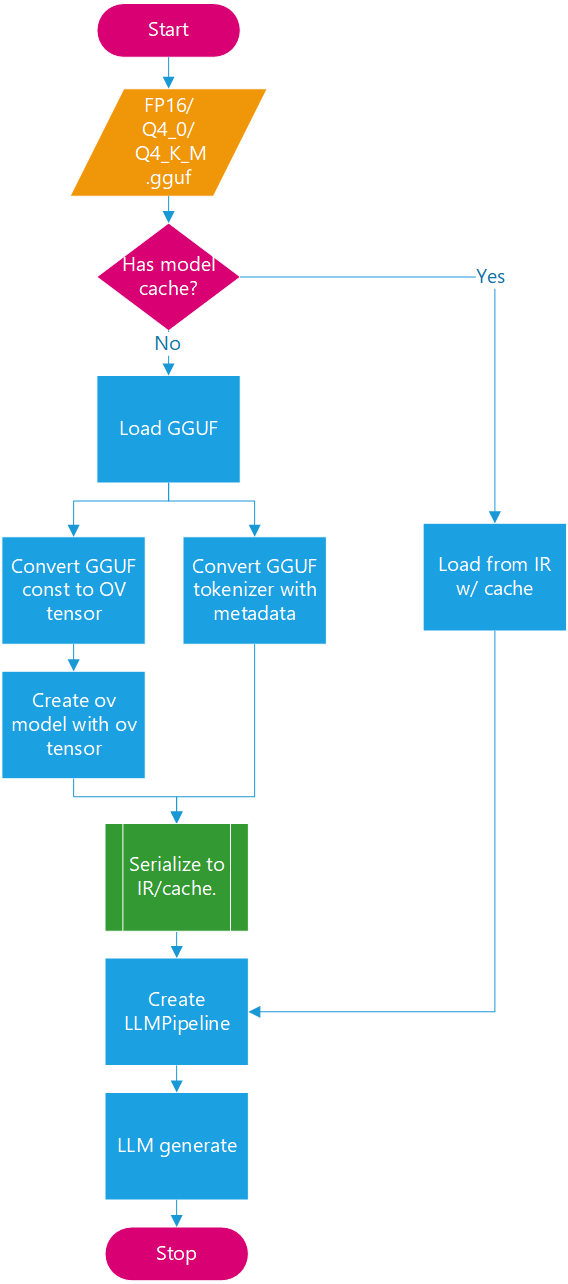
Future Architecture Workflow:
In GenAI 25.2, the LLMPipeline reads GGUF files during each initialization by default. In addition to supporting online tokenizer conversion, future updates will introduce optimizations to the GGUF LLMPipeline with configuration option to save converted OpenVINO models.
With the architecture defined, attention turns to the quantization formats.
To analyze the characteristics of Q4_K_M, it is helpful first to distinguish it from Q4_0, Q4_1, and Q8_0. These are lightweight, pure 4- or 8-bit quantization formats designed primarily for fast loading and minimal model size.
In contrast, Q4_K_M adopts a mixed-precision 4/6-bit scheme with a super-block structure that incorporates both block_scale and block_min, enabling higher accuracy while maintaining a compact footprint.
A deeper understanding of Q4_K_M can be achieved by comparing it directly with Q4_0. Notably, Q4_K_M encompasses two distinct GGUF tensor types: q4_k and q6_k. These tensors differ not only in precision but also in group size.
* Both Qwen2.5 Q4_0 and Q4KM GGUF have q6_k GGUF tensor. Q4_0 model’s last layer “output.weight” is the only one q6_k tensor.
-
So, what does this look like in practice? Qwen2.5 offers a clear example.
Qwen2.5 Q4_0 and Q4_K_M GGUF models both include q6_k tensors. In Q4_0, the only q6_k tensor is typically the final layer (output.weight). While OpenVINO shares embedding weights with lm_head, GGUF keeps them separate. For certain Qwen Q4_0 models (e.g., 3B/7B), lm_head is stored as a q6_k tensor in GGUF. To align with llama.cpp behavior and improve accuracy, this weight is loaded directly from GGUF instead of using shared embeddings.
Since INT6 is not supported by OpenVINO, all q6_k tensors are converted to INT8 for both Q4_0 and Q4_K_M models. Currently, to bypass GPU limitations with group-wise INT8 dequantization, q6_k tensors are converted to FP16 at load time on CPU. The q6_k workaround introduces some loading and inference performance overhead.
Q4_K_M models typically contain approximately six times more q4_k tensors than q6_k tensors. As a result, q6_k to fp16 workaround is relatively acceptable in terms of performance impact.
By leveraging common optimization techniques during the model loading phase, the overall pipeline latency can be further minimized.
Loading optimizations:
- - Parallel Parsing: Uses ov::parallel_for for multi-threaded.
- - Split-File Support: Compatible with llama.cpp’s sharding scheme for loading large GGUF models.
Loading performance results show that the Qwen2.5-7B-Q4_K_M model can be extracted and generated into an OpenVINO model graph in under 10 seconds on an Intel LNL U7 268V, dramatically outperforming the offline GGUF-to-OpenVINO approach, which takes about 4 minutes and over 15 GB of memory to save the PyTorch FP16 model (e.g., Llama-3.1-8b-Q4_K_M).
Dynamic shapes support in OpenVINO JIT compiler boosts inference performance by 40%
Authors: Ivan Novoselov, Alexandra Sidorova, Vladislav Golubev, Dmitry Gorokhov
Introduction
Deep learning (DL) has become a powerful tool for addressing challenges in various domains like computer vision, generative AI, and natural language processing. Industrial applications of deep learning often require performing inference in resource-constrained environments or in real time. That’s why it’s essential to optimize inference of DL models for particular use cases, such as low-latency, high-throughput or low-memory environments. Thankfully, there are several frameworks designed to make this easier, and OpenVINO stands out as a powerful tool for achieving these goals.
OpenVINO is an open-source toolkit for optimization and deployment of DL models. It demonstrates top-tier performance across a variety of hardware including CPU (x64, ARM), AI accelerators (Intel NPU) and Intel GPUs. OpenVINO supports models from popular AI frameworks and delivers out-of-the box performance improvements for diverse applications (you are welcome to explore demo notebooks). With ongoing development and a rapidly growing community, OpenVINO continues to evolve as a versatile solution for high-performance AI deployments.
The primary objective of OpenVINO is to maximize performance for a given DL model. To do that, OpenVINO applies a set of hardware-dependent optimizations The optimizations are typically performed by replacing a target group of operations with a custom operation that can be executed more efficiently. In the standard approach, these custom operations are executed using handcrafted implementations. This approach is highly effective when optimizing a few patterns of operations. On the other hand, it lacks scalability and thus requires too much effort when dozens of similar patterns should be supported.
To address this limitation and build a more flexible optimization engine, OpenVINO introduced Snippets, an integrated Just-In-Time (JIT) compiler for computational graphs. Snippets provide a flexible and scalable approach for operation fusions and enablement. The graph compiler automatically identifies subgraphs of operations that can benefit from fusion and combines them into a single node, referred to as “Subgraph”. Snippets then apply a series of optimizing transformations to the subgraph and JIT compile an executable that efficiently performs the computations defined by the subgraph.
One of the most common examples of such subgraphs is Scaled Dot-Product Attention (SDPA) pattern. SDPA it is a cornerstone of transformer-based architectures which dominate most of the state-of-the-art models. There are numerous SDPA pattern flavours and variations dictated by model-specific adjustments or optimizations. Thanks to compiler-based design, Snippets support most of these configurations. Fig. 1 illustrates the general structure of the SDPA pattern supported by Snippets, highlighting its adaptability to different model requirements:
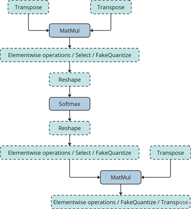
Note that SDPA has quadratic time and memory complexity with respect to sequence length. It means that by fusing SDPA-like patterns, Snippets significantly reduce memory consumption and accelerate transformer models, especially for large sequence lengths.
Snippets effectively optimized SDPA patterns but had a key limitation: they did not support dynamic shapes. In other words, input shapes must be known at the model compilation stage and can’t be changed in runtime. This limitation reduced the applicability of Snippets to many real-world scenarios where input shapes are not known in advance. While it is technically possible to JIT-compile a new binary for each unique set of input shapes, this approach introduces significant recompilation overheads, often negating the performance gains from SDPA fusion.
Fortunately, this static-shape limitation is not inherent to Snippets design. They can be modified to support dynamic shapes internally and generate shape-agnostic binaries. In this post, we discuss Snippets architecture and the challenges we faced during this dynamism enablement.
Architecture
The first step of the Snippets pipeline is called Tokenization. It is applied to an ov::Model, which represents OpenVINO Intermediate Representation (IR). It’s a standard IR in the OV Runtime you can read more about it here or here. The purpose of this stage is to identify parts of the initial model that can be lowered by Snippets efficiently. We are not going to discuss Tokenization in detail because this article is mostly focused on the dynamism implementation. A more in-depth description of the Tokenization process can be found in the Snippets design guide. The key takeaway for us here is that the subsequent lowering is performed on a part of the initial ov::Model. We will call this part Subgraph, and the Subgraph at first is also represented as an ov::Model.
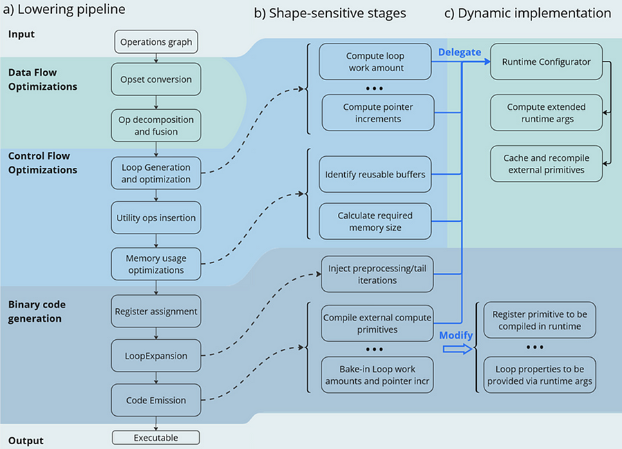
Now let’s have a look at the lowering pipeline, its schematic representation is shown on Fig.2a. As can be seen from the picture, the lowering process consists of three main phases: Data Flow Optimizations, Control Flow Optimizations and Binary Code Generation. Let’s briefly discuss each of them.
Lowering Pipeline
The first stage is the Data Flow optimizations. As we mentioned above, this stage’s input is a part of the initial model represented as an ov::Model. This representation is very convenient for high-level transformations such as opset conversion, operations’ fusion/decomposition and precision propagation. Here are some examples of the transformations performed on this stage:
- ConvertPowerToPowerStatic — operation Power with scalar exponent input is converted to PowerStatic operation from the Snippets opset. The PowerStatic ops then use the values of the exponents to produce more optimal code.
- FuseTransposeBrgemm — Transpose operations that can be executed in-place with Brgemm blocks are fused into the Brgemm operations.
- PrecisionPropagation pass automatically inserts Converts operations between the operations that don’t natively support the desired execution precision.
The next stage of the lowering process is Control Flow optimizations (or simply CFOs). Note that the ov::Model is designed to primarily describe data flow, so is not very convenient for CFOs. Therefore, we had to develop our own IR (called Linear IR or simply LIR) that explicitly represents both control and data flows, you can read more about LIR here. So the ov::Model IR is converted to LIR before the start of the CFOs.
As you can see from the Fig.2a, the Control Flow optimization pipeline could roughly be divided into three main blocks. The first one is called Loop Generation and Optimization. This block includes all loop-related optimizations such as automatic generation of loops based on the input tensors’ dimensions, loop fusion and blocking loops generation.
The second block of Control Flow optimizations is called Utility Ops Insertion. We need this block of transformations here to insert utility operations that depend on loop control structures, specifically on their entry and exit points locations. For example, operations like Load, Store, MemoryBuffer, LoopBegin and LoopEnd are inserted during this stage.
The last step of CFO is the Memory Usage Optimizations block. These transformations determine required sizes of internal memory buffers, and analyze how much of that memory can be reused. A graph coloring algorithm is employed to minimize memory consumption.
Now all Control Flow optimizations are performed, and we are ready to proceed to the next stage of the lowering pipeline — Binary Code Generation (BCG). As one can see from Fig.2a, this stage consists of three substages. The first one is Register Assignment. We use a fairly standard approach here: calculate live intervals first and use the linear scan algorithm to assign abstract registers that are later mapped to physical ones.
The next BSG substage is Loop Expansion. To better understand its purpose, let’s switch gears for a second and think about loops in general. Sometimes it’s necessary to process the first or the last iteration of a loop in a special way. For example, to initialize a variable or to process blocking loops’ tails. The Loop Expansion pass unrolls these special iterations (usually the first or the last one) and explicitly injects them into the IR. This is needed to facilitate subsequent code emission.
The final step of the BCG stage is Code Emission. At this stage, every operation in our IR is mapped to a binary code emitter, which is then used to produce a piece of executable code. As a result, we produce an executable that performs calculations described by the initial input ov::Model.
Dynamic Shapes Support
Note that some stages of the lowering pipeline are inherently shape-sensitive, i.e. they rely on specific values of input shapes to perform optimizations. These stages are schematically depicted on the Fig. 2b.
As can be seen from the picture, shapes are used to determine loops’ work amounts and pointer increments that should be performed on every iteration. These parameters are later baked into the executable during Code Emission. Another example is Memory Usage Optimizations, since input shapes are needed to calculate memory consumption. Loop Expansion also relies on input shapes, since it needs to understand if tail processing is required for a particular loop. Note also that Snippets use compute primitives from third-party libraries, BRGEMM block from OneDNN for example. These primitives should as well be compiled with appropriate parameters that are also shape-sensitive.
One way to address these challenges is to rerun the lowering pipeline for every new set of input shapes, and to employ caching to avoid processing the same shapes twice. However, preliminary analysis indicated that this approach is too slow. Since this re-lowering needs to be performed in runtime, the performance benefit provided by Snippets is essentially eliminated by the recompilation overheads.
The performed experiments thus indicate that we can afford to run the whole lowering pipeline only once during the model compilation stage. Only some minor adjustments can be made at runtime. In other words, we need to remove all shape-sensitive logic from the lowering pipeline and perform the compilation without it. The remaining shape-sensitive transformations should be performed at runtime. Of course, we would also need to share this runtime context with the compiled shape-agnostic kernel. The idea behind this approach is schematically represented on Fig. 2c.
As one can see from the picture, all the shape-sensitive transformations are now performed by a new entity called Runtime Configurator. It’s probably easier to understand its purpose in some examples.
Imagine that we need to perform a unary operation get_result(X) on an input tensor X — for example, apply an activation function. To do this, we need to load some input data from memory into registers, perform the necessary computations and write the results back to memory. Of course this read-compute-write sequence should be done in a loop since we need to process the entire input tensor. These steps are described in more detail in Fig. 3 using pseudocode. Fig. 3a corresponds to a static kernel while Fig. 3b represents a dynamic one.
Let’s consider the static kernel as a starting point. As the first step, we need to load pointers to input and output memory blobs to general-purpose registers (or simply GPRs) denoted G_IN and G_OUT on the picture. Then we initialize another GPR that stores the loop work amount (G_WA). Note that the loop is used to traverse the input tensor, so the loop’s work amount is fixed because the tensor’s dimensions are also known at the BCG stage. The next six steps in the picture (3 to 8) are in the loop’s body.
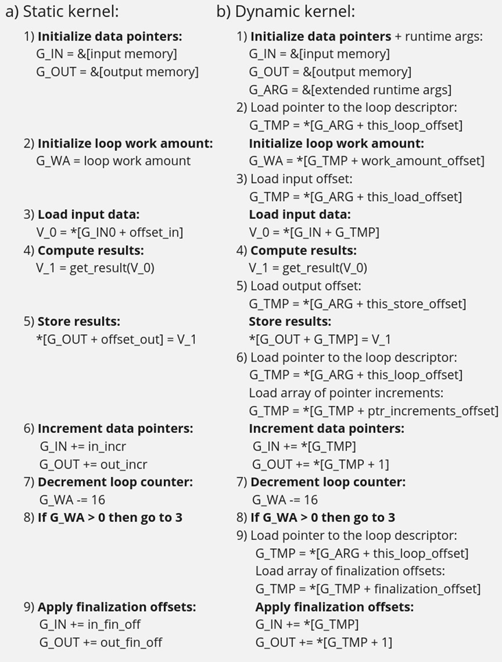
In step 3, we load input data into a vector register V_0, note that the appropriate pointer is already loaded to G_IN, and offset_in is fixed because the input tensor is static. Next, we apply our get_result function to the data in V_0 and place the result in a spare vector register V_1. Now we need to store V_1 back to memory, which is done on step 5. Note that offset_out is also known in the static case. This brings us almost to the end of the loop’s body, and the last few things we need to do are to increment data pointers (step 6), decrement loop counter (step 7), and jump to the beginning of the body, if needed (step 8).
Finally, we need to reset data pointers to their initial values after the loop is finished, which is done using finalization offsets on step 9. Note that this step could be omitted in our simplified example, but it’s often needed for more complicated use cases, such as when the data pointers are used by subsequent loops.
Now that we understand the static kernel, let’s consider the dynamic one, which is shown in Fig. 3b. Unsurprisingly, the dynamic kernel performs essentially the same steps as the static one, but with additional overhead due to loading shape-dependent parameters from the extended runtime arguments. Take step 1 as an example, we need to load not only memory pointers (to G_IN and G_OUT), but also a pointer to the runtime arguments prepared by the runtime configurator (to G_ARG).
Next, we need to load a pointer to the appropriate loop descriptor (a structure that stores loops’ parameters) to a temporary register G_TMP, and only then we can initialize the loop’s work amount register G_WA (step 2). Similarly, in order to load data to V_0, we need to load a runtime-calculated offset from the runtime arguments in step 3. The computations in step 4 are the same as in the static case, since they don’t depend on the input shapes. Storing the results to memory (step 5) requires reading a dynamic offset from the runtime arguments again. Next, we need to shift the data pointers, and again we have to load the increments from the corresponding loop descriptor in G_ARG because they are also shape-dependent, as the input tensor can be strided. The following two steps 7 and 8 are the same as in the static case, but the finalization offsets are also dynamic, so we have to load them from G_ARG yet again.
As one can see from Fig. 3, dynamic kernels incorporate additional overhead due to reading the extended runtime parameters provided by the runtime configurator. However, this overhead could be acceptable as long as the input tensor is large enough (Load/Store operations would take much longer than reading runtime arguments from L1) and the amount of computation is sufficient (get_results is much larger than the overhead). Let’s consider the performance of this design in the Results section to see if these conditions are met in practical use cases.
Results
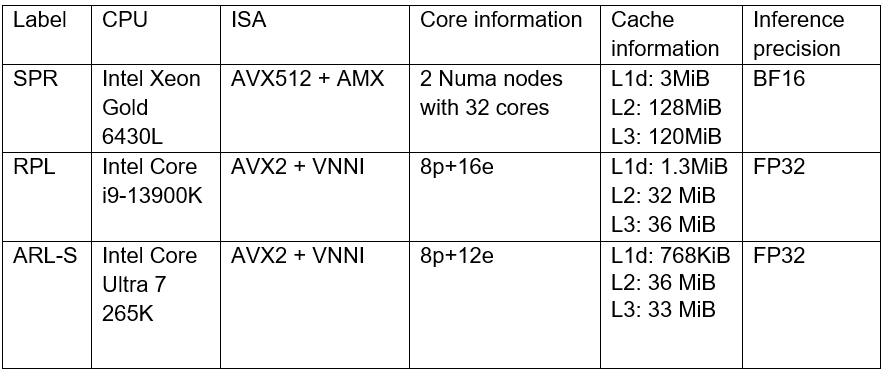
We selected three platforms to evaluate the dynamic pipeline’s performance in Snippets. These platforms represent different market segments: the Intel Core machine is designed for high-performance user and professional tasks. While the Intel Xeon is a good example of enterprise-level hardware often used in data centers and cloud computing applications. The information about the platforms is described in the table below:
As discussed in the Introduction, Snippets support various SDPA-like patterns which form the backbone of Transformer models. These models often work with input data of arbitrary size (for example, sequence length in NLP). Thus, dynamic shapes support in Snippets can efficiently accelerate many models based on Transformer architecture with dynamic inputs.
We selected 43 different Transformer-models from HuggingFace to measure how the enablement of dynamic pipeline in Snippets affects performance. The models were downloaded and converted to OpenVINO IRs using Optimum Intel. These models represent different domains and were designed to solve various tasks in natural language processing, text-to-image image generation and speech recognition (see full model list at the end of the article). What unifies all these models is that they all contain SDPA subgraph and thus can be accelerated by Snippets.
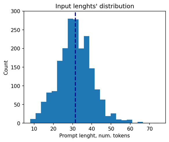
Let’s take a closer look at the selected models. The 37 models of them solve different tasks in natural language processing. Their performance was evaluated using a list of 2000 text sequences with different lengths, which also mimics the real-word scenario. The total processing time of all the sequences were measured in every experiment. Note that the text sequences were converted to model inputs using model-specific tokenizers prior to the benchmarking. The lengths’ distribution of the tokenized sequences is shown on Fig. 4. As can be seen from the picture, the distribution is close to normal with the mean length of 31 tokens.
The other 6 models of the selected model scope solve tasks in text-to-image image generation (Stable Diffusion) and speech recognition (Whisper). These models decompose into several smaller models after export to OpenVINO representation using Optimum Intel. Stable Diffusion topology is decomposed into Encoder, Diffuser and Decoder. The most interesting model here is Diffuser because it’s the one responsible for denoising of the latent image representation. This generation stage is repeated several times, so it is the most computationally intensive, which mostly effects on the generation time of the image. Whisper is also decomposed into Encoder and Decoder, which also contain SDPA patterns. The Encoder encodes the spectrogram from the feature extractor to form a sequence of encoder hidden states. Then, the decoder autoregressively predicts text tokens, conditional on both the previous tokens and the encoder hidden states. Currently, Snippets support efficient execution of SDPA only in Whisper Encoder, while Decoder is a subject for future support. To evaluate the inference performance of Stable Diffusion and Whisper models, we collect generation time of image/speech using LLM Benchmark from openvino.genai. This script provides a unified approach to estimate performance for GenAI workloads in OpenVINO.
Performance Improvements
Note that the main goal of these experiments is to estimate the impact of Snippets on the performance of the dynamic pipeline. To do that, we performed two series of experiments for every model. The first version of experiments is with disabled Snippets tokenization. In this case, all operations from the SDPA pattern are performed on the CPU plugin side as stand-alone operations. The second variant of experiments — with enabled Snippets tokenization. The relative difference between numbers collected on these two series of experiments is our performance metric — speedup, the higher the better. Firstly, let’s take a closer look at the resulting speedups for the BERT models which are depicted on Fig. 5.
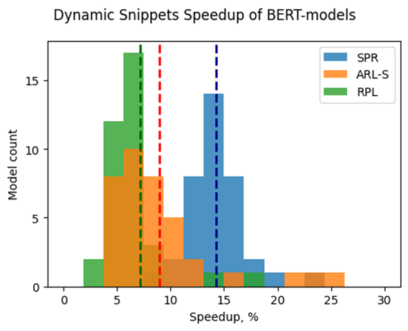
The speedups on RPL range from 3 to 18%, while on average the models are accelerated by 7%. The ARL-S speedups are somewhat higher and reach 20–25% for some models, the average acceleration factor is around 9%. The most affected platform is SPR, it has the highest average speedup of 15 %.
One can easily see from these numbers that both average and maximum speedups depend on the platform. To understand the reason for this variation, we should recall that the main optimizations delivered by Snippets are vertical fusion and tiling. These optimizations improve cache locality and reduce the memory access overheads. Note SPR has the largest caches among the examined platforms. It also uses BF16 precision that takes two times less space per data element compared to F32 used on ARL-S and RPL. Finally, SPR has AMX ISA extension that allows it to perform matrix multiplications much faster. As a result, SDPA execution was more memory bound on SPR, so this platform benefited the most from the Snippets enablement. At the same time, the model speedups on ARL-S and RPL are almost on the same level. These platforms use FP32 inference precision while SPR uses BF16, and they have less cache size than SPR.
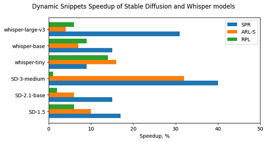
Now, let’s consider Stable Diffusion and Whisper topologies and compare their speedups with some of BERT-like models. As can be seen from the Fig. 6, the most accelerated Stable Diffusion topology is StableDiffusion-3-medium — almost 33% on ARL-S and 40% on SPR. The most accelerated model in this Stable Diffusion pipeline is Diffuser. This model has made a great contribution to speeding up the entire image generation time. The reason the Diffuser benefits more from Snippets enablement is that they use larger sequence lengths and embedding sizes. It means that their attention blocks process more data and are more memory constrained compared to BERT-like models. As a result, the Diffuser models in Stable Diffusion benefit more from the increased cache locality provided by Snippets. This effect is more pronounced on the SPR than on the ARL-S and RPL for the reasons discussed above (cache sizes, BF16, AMX).
The second most accelerated model is whisper-large-v3–30% on SPR. This model has more parameters than base and tiny models and process more Mel spectrogram frequency bins than they. It means that Encoder of whisper-large-v3 attention blocks processes more data, like Diffuser part of Stable Diffusion topologies. By the same reasons, whisper-large-v3 benefits more (increased cache locality provided by Snippets).
Memory Consumption Improvements
Another important improvement from Snippets using is reduction of memory consumption. Snippets use vertical fusion and various optimizations from Memory Usage Optimizations block (see the paragraph “Lowering Pipeline” in “Architecture” above for more details). Due to this fact, Subgraphs tokenized by Snippets consumes less memory than the same operations performed as stand-alone in CPU Plugin.
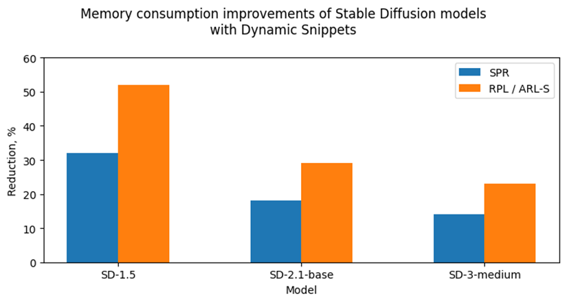
Let’s take a look at the Fig. 7 where we can see improvements in image generation memory consumption using Stable Diffusion pipelines from Snippets usage. As discussed above, the attention blocks in the Diffuser models from these pipelines process more data and consume more memory. Because of that, the greatest impact on memory consumption from using Snippets is seen on Stable Diffusion pipelines. For example, memory consumption of image generation is reduced by 25–50% on RPL and ARL-S platforms with FP32 inference precision and by 15–30% on SPR with BF16 inference precision.
Thus, one of the major improvements from using Snippets is memory consumption reduction. It allows extending the range of platforms which are capable to infer such memory-intensive models as Stable Diffusion.
Conclusion
Snippets is a JIT compiler used by OpenVINO to optimize performance-critical subgraphs. We briefly discussed Snippets’ lowering pipeline and the modifications made to enable dynamism support. After these changes, Snippets generate shape-agnostic kernels that can be used for various input shapes without recompilation.
This design was tested on realistic use cases across several platforms. As a result, we demonstrate that Snippets can accelerate BERT-like models by up to 25%, Stable Diffusion and Whisper pipelines up to 40%. Additionally, Snippets can significantly reduce memory consumption by several tens of percent. Notably, these improvements result from more optimal hardware utilization, so the models’ accuracy remains unaffected.
References
Model list can be found here: https://gist.github.com/a-sidorova/2c2aa584922389138e5ccbad0e0c773b
Intel Xeon Gold 6430L: https://www.intel.com/content/www/us/en/products/sku/231737/intel-xeon-gold-6430-processor-60m-cache-2-10-ghz/specifications.html
Intel Core i9-13900K: https://www.intel.com/content/www/us/en/products/sku/230496/intel-core-i913900k-processor-36m-cache-up-to-5-80-ghz/specifications.html
Intel Core Ultra 7 265K: https://www.intel.com/content/www/us/en/products/sku/241063/intel-core-ultra-7-processor-265k-30m-cache-up-to-5-50-ghz/specifications.html
Notices & Disclaimers
Performance varies by use, configuration, and other factors. Learn more on the Performance Index site.
No product or component can be absolutely secure. Your costs and results may vary. Intel technologies may require enabled hardware, software or service activation.
© Intel Corporation. Intel, the Intel logo, and other Intel marks are trademarks of Intel Corporation or its subsidiaries.
OpenVINO.GenAI Delivers C API for Seamless Language Interop with Practical Examples in .NET
Authors: Tong Qiu, Xiake Sun
Starting with OpenVINO.GenAI 2025.1, the C API has been introduced, primarily to enhance interoperability with other programming languages, enabling developers to more effectively utilize OpenVINO-based generative AI across diverse coding environments.
Compared to C++, C's ABI is more stable, often serving as an interface layer or bridge language for cross-language interoperability and integration. This allows developers to leverage the performance benefits of C++ in the backend while using other high-level languages for easier implementation and integration.
As a milestone, we have currently delivered only the LLMPipeline and its associated C API interface. If you have other requirements or encounter any issues during usage, please submit an issue to OpenVINO.GenAI
Currently, we have implemented a Go application Ollama using the C API (Please refer to https://blog.openvino.ai/blog-posts/ollama-integrated-with-openvino-accelerating-deepseek-inference), which includes more comprehensive features such as performance benchmarking for developers reference.
Now, let's dive into the design logic of the C API, using a .NET C# example as a case study, based on the Windows platform with .NET 8.0.
Live Demo
Before we dive into the details, let's take a look at the final C# version of the ChatSample, which supports multi-turn conversations. Below is a live demo
How to Build a Chat Sample by C#
P/Invoke: Wrapping Unmanaged Code in .NET
First, the official GenAI C API can be found in this folder https://github.com/openvinotoolkit/openvino.genai/tree/master/src/c/include/openvino/genai/c . We also provide several pure C samples https://github.com/openvinotoolkit/openvino.genai/tree/master/samples/c/text_generation . Now, we will build our own C# Chat Sample based on the chat_sample_c. This sample can facilitate multi-turn conversations with the LLM.
C# can access structures, functions and callbacks in the unmanaged library openvino_genai_c.dll through P/Invoke. This example demonstrates how to invoke unmanaged functions from managed code.
public static class NativeMethods
{
 DllImport("openvino_genai_c.dll", CallingConvention = CallingConvention.Cdecl)]
public static extern ov_status_e ov_genai_llm_pipeline_create(
        [MarshalAs(UnmanagedType.LPStr)] string models_path,
        [MarshalAs(UnmanagedType.LPStr)] string device,
        out IntPtr pipe);

[DllImport("openvino_genai_c.dll", CallingConvention = CallingConvention.Cdecl)]
public static extern void ov_genai_llm_pipeline_free(IntPtr pipeline);

//Other methods
The dynamic library openvino_genai_c.dll is imported, which relies on openvino_genai.dll. CallingConvention = CallingConvention.Cdecl here corresponds to the default calling convention _cdecl in C, which defines the argument-passing order, stack-maintenance responsibility, and name-decoration convention. For more details, refer to Argument Passing and Naming Conventions.
Additionally, the return value ov_status_e reuses an enum type from openvino_c.dll to indicate the execution status of the function. We need to implement a corresponding enum type in C#, such as
public enum ov_status_e
{
    OK = 0,
    GENERAL_ERROR = -1,
    NOT_IMPLEMENTED = -2,
    //...

}
Next, we will implement our C# LLMPipeline, which inherits the IDisposable interface. This means that its instances require cleanup after use to release the unmanaged resources they occupy. In practice, object allocation and deallocation for native pointers are handled through the C interface provided by OpenVINO.GenAI. The OpenVINO.GenAI library takes full responsibility for memory management, which ensures memory safety and eliminates the risk of manual memory errors.
public class LlmPipeline : IDisposable
{
    private IntPtr _nativePtr;

    public LlmPipeline(string modelPath, string device)
    {
        var status = NativeMethods.ov_genai_llm_pipeline_create(modelPath, device, out _nativePtr);
        if (_nativePtr == IntPtr.Zero || status != ov_status_e.OK)
        {
            Console.WriteLine($"Error: {status} when creating LLM pipeline.");
            throw new Exception("Failed to create LLM pipeline.");
        }

        Console.WriteLine("LLM pipeline created successfully!");
    }

    public void Dispose()
    {
        if (_nativePtr != IntPtr.Zero)
        {
            NativeMethods.ov_genai_llm_pipeline_free(_nativePtr);
            _nativePtr = IntPtr.Zero;
        }

        GC.SuppressFinalize(this);
    }
    // Other Methods
}
Callback Implementation
Next, let's implement the most complex method of the LLMPipeline, the GenerateStream method. This method encapsulates the LLM inference process. Let's take a look at the original C code. The result can be retrieved either via ov_genai_decoded_results or streamer_callback. ov_genai_decoded_results provides the inference result all at once, while streamer_callback allows for streaming inference results. ov_genai_decoded_results or streamer_callback must be non-NULL; neither can be NULL at the same time. For more information please refer to the comments https://github.com/openvinotoolkit/openvino.genai/blob/master/src/c/include/openvino/genai/c/llm_pipeline.h
// code snippets from //https://github.com/openvinotoolkit/openvino.genai/blob/master/src/c/include/openvino/genai/c/llm_// pipeline.h
typedef enum {
    OV_GENAI_STREAMMING_STATUS_RUNNING = 0,  // Continue to run inference
    OV_GENAI_STREAMMING_STATUS_STOP =
        1,  // Stop generation, keep history as is, KV cache includes last request and generated tokens
    OV_GENAI_STREAMMING_STATUS_CANCEL = 2  // Stop generate, drop last prompt and all generated tokens from history, KV
                                           // cache includes history but last step
} ov_genai_streamming_status_e;

// ...
typedef struct {
    ov_genai_streamming_status_e(
        OPENVINO_C_API_CALLBACK* callback_func)(const char* str, void* args);  //!< Pointer to the callback function
    void* args;  //!< Pointer to the arguments passed to the callback function
} streamer_callback;

// ...
OPENVINO_GENAI_C_EXPORTS ov_status_e ov_genai_llm_pipeline_generate(ov_genai_llm_pipeline* pipe,
                                                                    const char* inputs,
                                                                    const ov_genai_generation_config* config,
                                                                    const streamer_callback* streamer,
                                                                    ov_genai_decoded_results** results);
The streamer_callback structure includes not only the callback function itself, but also an additional void* args for enhanced flexibility. This design allows developers to pass custom context or state information to the callback.
For example, in C++ it's common to pass a this pointer through args, enabling the callback function to access class members or methods when invoked.
// args is a this pointer
void callback_func(const char* str, void* args) {
    MyClass* self = static_cast<MyClass*>(args);
    self->DoSomething();
}
This C# code defines a class StreamerCallback that helps connect a C callback function with a C# method. It wraps a C function pointer MyCallbackDelegate and a void* args into a struct.
- ToNativePTR method constructs the streamer_callback structure, allocates a block of memory, and copies the structure's data into it, allowing it to be passed to a native C function.
- GCHandle is used to safely pin the C# object so that it can be passed as a native pointer to unmanaged C code.
- CallbackWrapper method is the actual function that C code will call.
[UnmanagedFunctionPointer(CallingConvention.Cdecl)]
public delegate ov_genai_streamming_status_e MyCallbackDelegate(IntPtr str, IntPtr args);

[StructLayout(LayoutKind.Sequential)]
public struct streamer_callback
{
    public MyCallbackDelegate callback_func;
    public IntPtr args;
}
public class StreamerCallback : IDisposable
{
    public Action<string> OnStream;
    public MyCallbackDelegate Delegate;
    private GCHandle _selfHandle;

    public StreamerCallback(Action<string> onStream)
    {
        OnStream = onStream;
        Delegate = new MyCallbackDelegate(CallbackWrapper);
        _selfHandle = GCHandle.Alloc(this);
    }

    public IntPtr ToNativePtr()
    {
        var native = new streamer_callback
        {
            callback_func = Delegate,
            args = GCHandle.ToIntPtr(_selfHandle)
        };

        IntPtr ptr = Marshal.AllocHGlobal(Marshal.SizeOf<streamer_callback>());
        Marshal.StructureToPtr(native, ptr, false);
        return ptr;
    }

    public void Dispose()
    {
        if (_selfHandle.IsAllocated)
            _selfHandle.Free();
    }

    private ov_genai_streamming_status_e CallbackWrapper(IntPtr str, IntPtr args)
    {
        string content = Marshal.PtrToStringAnsi(str) ?? string.Empty;

        if (args != IntPtr.Zero)
        {
            var handle = GCHandle.FromIntPtr(args);
            if (handle.Target is StreamerCallback self)
            {
                self.OnStream?.Invoke(content);
            }
        }

        return ov_genai_streamming_status_e.OV_GENAI_STREAMMING_STATUS_RUNNING;
    }
}
Then We implemented the GenerateStream method in class LLMPipeline.
 public void GenerateStream(string input, GenerationConfig config, StreamerCallback? callback = null)
 {
     IntPtr configPtr = config.GetNativePointer();
     IntPtr decodedPtr;// placeholder

     IntPtr streamerPtr = IntPtr.Zero;

     if (callback != null)
     {
         streamerPtr = callback.ToNativePtr();
     }

     var status = NativeMethods.ov_genai_llm_pipeline_generate(
         _nativePtr,
         input,
         configPtr,
         streamerPtr,
         out decodedPtr
     );

     if (streamerPtr != IntPtr.Zero)
         Marshal.FreeHGlobal(streamerPtr);

     callback?.Dispose();

     if (status != ov_status_e.OK)
     {
         Console.WriteLine($"Error: {status} during generation.");
         throw new Exception("Failed to generate results.");
     }
     return;
 }
We use the following code to invoke our callback and GenerateStream.
pipeline.StartChat(); // Start chat with keeping history in kv cache.

Console.WriteLine("question:");
while (true)
{
    string? input = Console.ReadLine();
    if (string.IsNullOrWhiteSpace(input)) break;

    using var streamerCallback = new StreamerCallback((string chunk) =>
    {
        Console.Write(chunk);
    });

    pipeline.GenerateStream(input, generationConfig, streamerCallback);

    input = null;
    Console.WriteLine("\n----------\nquestion:");
}

pipeline.FinishChat(); // Finish chat and clear history in kv cache.
About Deployment
We can directly download the OpenVINO official release of the LLM's IR from Hugging Face using this link.
git clone https://huggingface.co/OpenVINO/Phi-3.5-mini-instruct-int8-ov
The OpenVINO.GenAI 2025.1 package can be downloaded via this link.
The C# project directly depends on openvino_genai_c.dll, which in turn has transitive dependencies on other toolkit-related DLLs, including Intel TBB libraries.
To ensure proper runtime behavior, all the DLLs delivered with OpenVINO.GenAI — including openvino_genai_c.dll and its dependencies — are bundled and treated as part of the C# project’s runtime dependencies.
We use the following cmd commands to download the genai package and copy all the required dependent DLLs to the directory containing the *.csproj file.
curl -O https://storage.openvinotoolkit.org/repositories/openvino_genai/packages/2025.1/windows/openvino_genai_windows_2025.1.0.0_x86_64.zip
tar -xzvf openvino_genai_windows_2025.1.0.0_x86_64.zip
xcopy /y openvino_genai_windows_2025.1.0.0_x86_64\runtime\bin\intel64\Release\*.dll "C:\path\to\ChatSample\"
xcopy /y openvino_genai_windows_2025.1.0.0_x86_64\runtime\3rdparty\tbb\bin\*.dll "C:\path\to\ChatSample\"
Full Implementation
Please refer to https://github.com/apinge/openvino_ai_practice/tree/main/ov_genai_interop/ov_genai_interop_net, to access the full implementation.
Q1'25: Technology Update – Low Precision and Model Optimization
Authors
Alexander Kozlov, Nikolay Lyalyushkin, Nikita Savelyev, Souvikk Kundu, Andrey Anufriev, Pablo Munoz, Alexander Suslov, Liubov Talamanova, Daniil Lyakhov, Yury Gorbachev, Nilesh Jain, Maxim Proshin, Evangelos Georganas
Summary
This quarter we noticed a significant effort and progress on optimizing LLMs for long-context tasks. The current trend is that each and every LLM is published with the extended (usually interpolated) context which is usually 128K and above. The idea is to naturally process large amount of data within the model instead of preprocess it the way RAG systems do it. It inevitably increases computational complexity specifically of ScaledDotProductAttention operation which gets dominant on long contexts. Thus, many works devoted to the optimization of rather prefill with special computation patterns (A-shape, Tri-shape, XAttention) or using Sparse Attention at the decoding stage.
Highlights
- ParetoQ: Scaling Laws in Extremely Low-bit LLM Quantization by Meta (https://arxiv.org/pdf/2502.02631). The paper presents a unified framework that facilitates comparisons across 1-bit, 1.58-bit, 2-bit, 3-bit, and 4-bit quantization settings. The findings reveal a notable learning transition between 2 and 3 bits: For 3-bits and above, the fine-tuned models stay close to their original pre-trained distributions, whereas for learning 2-bit networks or below, the representations change drastically. By optimizing training schemes and refining quantization functions, the ternary 600M-parameter model even outperforms the previous SoTA ternary 3B-parameter model in accuracy, using only one-fifth of the parameters.
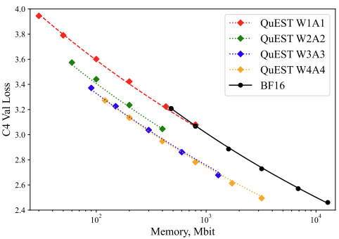
- QuEST: Stable Training of LLMs with 1-Bit Weights and Activations by ISTA and Red Hat AI (https://arxiv.org/pdf/2502.05003). The paper introduces quantization method that allows stable training with 1-bit weights and activations. It achieves this by improving two key aspects of QAT methods: (1) accurate and fast quantization of the (continuous) distributions of weights and activations via Hadamard normalization and MSE-optimal fitting; (2) a new trust gradient estimator based on the idea of explicitly minimizing the error between the noisy gradient computed over quantized states and the “true” (but unknown) full-precision gradient. Experiments on Llama-type architectures show that the method induces stable scaling laws across the entire range of hardware-supported precisions, and can be extended to sparse representations. The code is available at https://github.com/IST-DASLab/QuEST.
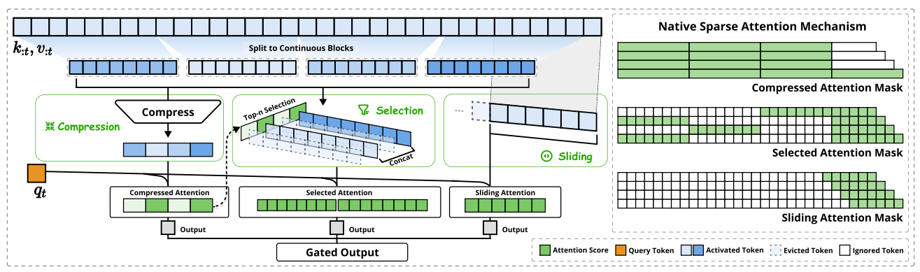
- Native Sparse Attention: Hardware-Aligned and Natively Trainable Sparse Attention by Deepseek-AI, Peking University, University of Washington (https://arxiv.org/pdf/2502.11089). The paper presents a method with hardware-aligned optimizations to achieve efficient long-context modeling. It employs a dynamic hierarchical sparse strategy, combining coarse-grained token compression with fine-grained token selection to preserve both global context awareness and local precision. The approach advances sparse attention design with two key features: (1) Authors achieve substantial speedups through arithmetic intensity-balanced algorithm design, with implementation optimizations for modern hardware. (2) They enable end-to-end training, reducing pretraining computation without sacrificing model performance. Experiments show the model pretrained with the proposed method maintains or exceeds Full Attention models across general benchmarks, long-context tasks, and instruction-based reasoning. It achieves substantial speedups over Full Attention on 64k-length sequences across decoding, forward propagation, and backward propagation. Non-official implementations are available on GitHub.
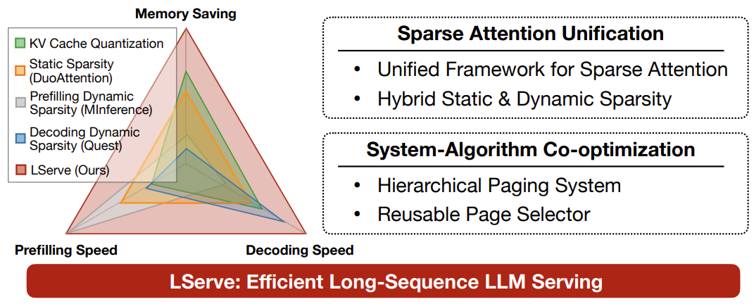
- LSERVE: EFFICIENT LONG-SEQUENCE LLM SERVING WITH UNIFIED SPARSE ATTENTION by MIT, SJTU, Nvidia (https://arxiv.org/pdf/2502.14866). The paper introduces a system that accelerates long-sequence LLM serving via hybrid sparse attention. This method unifies different hardware-friendly, structured sparsity patterns for both prefilling and decoding attention into a single framework, where computations on less important tokens are skipped block-wise. It demonstrates the compatibility of static and dynamic sparsity in long-context LLM attention. Authors convert half of the attention heads to nearly free streaming heads in both the prefilling and decoding stages. Additionally, we they that only a constant number of KV pages is required to preserve long-context capabilities, irrespective of context length. They then design a hierarchical KV page selection policy that dynamically prunes KV pages based on query-centric similarity. The method accelerates LLM prefilling by up to 2.9x and decoding by 1.3-2.1x over vLLM, maintaining long-context accuracy. Code is released at https://github.com/mit-han-lab/omniserve.
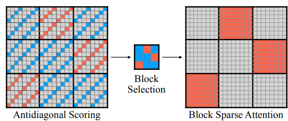
- XAttention: Block Sparse Attention with Antidiagonal Scoring by Tsinghua University, MIT, SJTU, and NVIDIA (https://arxiv.org/pdf/2503.16428). The paper introduces XAttention method that significantly accelerates long-context inference in Transformers models using sparse attention. XAttention’s key innovation is the insight that the sum of antidiagonal values (i.e., from the lower-left to upper-right) in the attention matrix provides a powerful proxy for block importance. This allows for precise identification and pruning of non-essential blocks, resulting in high sparsity and dramatically accelerated inference. On RULER and LongBench for language, VideoMME for video understanding, and VBench for video generation—XAttention achieves accuracy comparable to full attention while delivering substantial computational gains. It shows up to 13.5x acceleration in attention computation. The code is available at https://github.com/mit-han-lab/x-attention.
Papers with notable results
Quantization
- Optimizing Large Language Model Training Using FP4 Quantization by Microsoft and University of Science and Technology of China (https://arxiv.org/pdf/2501.17116). The work introduces the FP4 training framework for LLMs, addressing quantization challenges with two key ideas: a differentiable quantization estimator for precise weight updates and an outlier clamping and compensation strategy to prevent activation collapse. To ensure stability, the framework integrates a mixed-precision training scheme and vector-wise quantization. Experimental results demonstrate that our FP4 framework achieves accuracy comparable to BF16 and FP8, with minimal degradation, scaling effectively to 13B-parameter LLMs trained on up to 100B.
- MQuant: Unleashing the Inference Potential of Multimodal Large Language Models via Full Static Quantization by Houmo AI, Southeast University, and Xi’an Jiaotong University (https://arxiv.org/pdf/2502.00425). The work focuses on the problems of VLM quantization with a coarse scale granularity. It proposes several techniques to tackle the quantization problems, namely: Modality-Specific Static Quantization (MSQ), assigning distinct static scales for visual vs. textual tokens; Attention-Invariant Flexible Switching (AIFS), reordering tokens to preserve casual attention while eliminating expensive token-wise scale computations; Rotation Magnitude Suppression (RMS), mitigating weight outliers arising from online Hadamard rotations. On five mainstream VLMs (including Qwen-VL, MiniCPM-V, CogVLM2), the method achieves near-floating-point accuracy under W4A8 setting. The code is planned to be published.
- An Empirical Study of LLaMA3 Quantization: From LLMs to MLLMs by The University of Hong Kong, Beihang University, and ETH Zurich (https://arxiv.org/pdf/2404.14047). Authors assessed the performance of the LLaMA3-based LLaVA-Next-8B model under 2-4 ultra-low bits with post-training quantization methods. Experimental results indicate that LLaMA3 still suffers from non-negligible degradation in linguistic and visual contexts, particularly under ultra-low bit widths. This highlights the significant performance gap at low bit-width that needs to be addressed in future developments. The code is available at: https://github.com/Macaronlin/LLaMA3-Quantization.
- Nanoscaling Floating-Point (NxFP): NanoMantissa, Adaptive Microexponents, and Code Recycling for Direct-Cast Compression of Large Language Models by Harvard University (https://arxiv.org/pdf/2412.19821). This paper profiles modern LLMs and identifies three main challenges of low-bit Microscaling format, i.e., inaccurate tracking of outliers, vacant quantization levels, nd wasted binary code. In response, Nanoscaling (NxFP) proposes three techniques, i.e., NanoMantissa, Adaptive Microexponent, and Code Recycling to enable better accuracy and smaller memory footprint than state-of-the-art MxFP. Experimental results on direct-cast inference across various modern LLMs demonstrate that the proposed methods outperform MxFP by up to 0.64 in perplexity and by up to 30% in accuracy on MMLU benchmarks.
- RoSTE: An Efficient Quantization-Aware Supervised Fine-Tuning Approach for Large Language Models by University of Minnesota and The Chinese University of Hong Kong (https://arxiv.org/pdf/2502.09003). The paper introduces a fine-tuning based method that directly optimizes quantized weights and rotation matrices within a single model architecture. It proposes a bilevel optimization formulation, where upper level subproblem optimizes weight matrices, while lower level subproblem employs a surrogate loss to guide the selection of rotation matrix. Authors designed an algorithm which alternates between (i) a QAT subroutine incorporating a rotation-enabled straightthrough-estimator (STE) update, and (ii) a low complexity heuristic for selecting rotation matrices based on the random Walsh-Hadamard matrix. They provide a theoretical analysis of the benefits of rotation-enabled quantization in QA-SFT by examining the prediction error resulted from the QAT stage of RoSTE. This analysis directly motivates the use of quantization error based surrogate loss and justifies the adoption.
- NESTQUANT: NESTED LATTICE QUANTIZATION FOR MATRIX PRODUCTS AND LLMS by MIT and Hebrew University of Jerusalem (https://arxiv.org/pdf/2502.09720). The paper proposes a PTQ scheme for weights and activations that is based on self-similar nested lattices. Recent work has mathematically shown such quantizers to be information-theoretically optimal for low-precision matrix multiplication. We implement a practical low-complexity version based on Gosset lattice, making it a drop-in quantizer for any matrix multiplication step (e.g., in self-attention, MLP etc). For example, the method quantizes weights, KV-cache, and activations of Llama-3-8B to 4 bits, achieving perplexity of 6.6 on wikitext2.
- ViM-VQ: Efficient Post-Training Vector Quantization for Visual Mamba by Zhejiang University and vivo Mobile (https://arxiv.org/pdf/2503.09509). A practical study of vector quantization method for Visual Mamba networks (ViMs). Authors identify several key challenges: 1) The weights of Mamba-based blocks in ViMs contain numerous outliers, significantly amplifying quantization errors. 2) When applied to ViMs, the latest VQ methods suffer from excessive memory consumption, lengthy calibration procedures, and suboptimal performance in the search for optimal codewords. They propose a post-training vector quantization method tailored for ViMs. It consists of two components: 1) a fast convex combination optimization algorithm that updates both the convex combinations and the convex hulls to search for optimal codewords, and 2) an incremental vector quantization strategy that incrementally confirms optimal codewords to mitigate truncation errors. The results demonstrate that the method achieves stateof-the-art performance in low-bit quantization across various visual tasks.
- SSVQ: Unleashing the Potential of Vector Quantization with Sign-Splitting by Zhejiang University and vivo Mobile (https://arxiv.org/pdf/2503.08668). The paper proposes the vector quantization approach which decouples the sign bit of weights from the codebook. It involves extracting the sign bits of uncompressed weights and performing clustering and compression on all-positive weights. Authors also introduce latent variables for the sign bit and jointly optimize both the signs and the codebook. Additionally, they implement a progressive freezing strategy for the learnable sign to ensure training stability. Experiments on modern models and tasks demonstrate that the method achieves a good compression-accuracy trade-off compared to conventional VQ. Authors also validate the algorithm on a hardware accelerator, showing that SSVQ achieves a 3× speedup over the 8-bit compressed model by reducing memory access.
- MergeQuant: Accurate 4-bit Static Quantization of Large Language Models by Channel-wise Calibration (https://arxiv.org/pdf/2503.07654). The paper introduces per-channel static quantization method. It integrates the per-channel quantization steps with the corresponding scalings and linear mappings through a Quantization Step Migration method, eliminating the quantization overheads before and after matrix multiplication. Authors also propose dimensional reconstruction and adaptive clipping to address the nonuniformity of quantization scale factors and redistribute the channel variations to the subsequent modules to balance the parameter distribution under QSM. They evaluate method on Llama 2 and Llama 3 models in W4A4 setting.
- QuantCache: Adaptive Importance-Guided Quantization with Hierarchical Latent and Layer Caching for Video Generation by Shanghai Jiao Tong University, MGTV, Shanhai Academy (https://arxiv.org/pdf/2503.06545). Authors propose a training-free inference acceleration framework that jointly optimizes hierarchical latent caching, adaptive importance-guided quantization, and structural redundancy-aware pruning. It achieves an end-to-end latency speedup of 6.72x on OpenSora with minimal loss in generation quality. experiments across multiple video generation benchmarks demonstrate the effectiveness of our method for DiT inference. The code and models will be available at https://github.com/JunyiWuCode/QuantCache.
- Matryoshka Quantization by Google DeepMind (https://arxiv.org/pdf/2502.06786). Practitioners are often forced to maintain multiple models with different quantization levels or serve a single model that best satisfies the quality-latency trade-off. On the other hand, integer data types, such as int8, inherently possess a nested (Matryoshka) structure where smaller bit-width integers, like int4 or int2, are nested within the most significant bits. In this paper, the authors propose Matryoshka Quantization (MatQuant), a multi-scale quantization technique that alleviates the aforementioned challenge. It allows us to train and maintain a single quantized model but serve it with the precision demanded by the deployment. Furthermore, leveraging MatQuant’s co-training and co-distillation regularization, int2 precision models extracted by MatQuant outperform standard int2 quantization by up to to 4% and 7% with OmniQuant and QAT as base algorithms respectively. Finally, authors demonstrate that by using an extra bit to represent outliers, a model with an effective precision of 2.05-bit gives an additional 6% improvement with OmniQuant as the base algorithm.
Pruning/Sparsity
- Mamba-Shedder: Post-Transformer Compression for Efficient Selective Structured State Space Models by Intel Labs (https://arxiv.org/pdf/2501.17088v1). This paper explores the compression of SSM-based models, particularly Mamba and its hybrids. The authors discuss the sensitivity of these models to the removal of selected components at different granularities to reduce the model size and computational overhead, thus improving their efficiency while maintaining accuracy. The proposed solutions, collectively referred to as Mamba-Shedder, achieve a speedup of up to 1.4x during inference, demonstrating that model efficiency can be improved by eliminating several redundancies with minimal impact on the overall model performance. The code is available at https://github.com/IntelLabs/Hardware-Aware-Automated-Machine-Learning.
- DeepSeekAI, The Sparsity Revolution That Shook the AI Market: https://www.linkedin.com/pulse/deepseek-ai-sparsity-revolution-shook-market-jabar-riaz-hwvbf. The blogpost discusses two types of sparsity to train efficient and competitive LLM models, namely data sparsity and model sparsity.
Other
- TPU Scaling Book from Google - a series of blog posts on how to optimize LLMs for Google TPUv5: https://jax-ml.github.io/scaling-book/applied-inference.
- The Ultra-Scale Playbook: Training LLMs on GPU Clusters https://huggingface.co/spaces/nanotron/ultrascale-playbook. A tutorial from HuggingFace on the basics of multi-GPU training and how to scale it.
- Qwen2.5-1M Technical Report by Alibaba (https://qianwen-res.oss-cn-beijing.aliyuncs.com/Qwen2.5-1M/Qwen2_5_1M_Technical_Report.pdf). Authors introduce Qwen2.5-1M, a series of models that extend the context length to 1 million tokens. Compared to the previous 128K version, the Qwen2.5-1M series has significantly enhanced long-context capabilities through long-context pretraining and post-training. To reduce inference costs, authors implement a sparse attention method along with chunked prefill optimization for deployment scenarios and a sparsity refinement method to improve precision. Additionally, they detail optimizations in the inference engine, including kernel optimization, pipeline parallelism, and scheduling optimization, which significantly enhance overall inference performance. Qwen2.5-1M models achieve a remarkable 3x to 7x prefill speedup in scenarios with 1 million tokens of context.
- WaferLLM: A Wafer-Scale LLM Inference System by University of Edinburgh and Microsoft (https://arxiv.org/pdf/2502.04563). The paper introduces LLM inference system that is guided by a device model that captures the unique hardware characteristics of wafer-scale architectures. It proposes MeshGEMM and MeshGEMV, the GEMM and GEMV implementations designed to scale effectively on wafer-scale accelerator. Authors focus on four principles when designing the implementation: Massive Parallel cores, Highly non-uniform memory access Latency, Constrained local Memory, and Limited hardware-assisted Routing. Evaluations show that the method achieves 200× better wafer-scale accelerator utilization than state-of-the-art systems. On a commodity wafer-scale accelerator, it delivers 606× faster and 22× more energy-efficient GEMV compared to an advanced GPU. One of the limitations of the method is a limited model size due to a need to replicate memory over the computational units to increase the latency.
- EmbBERT-Q: Breaking Memory Barriers in Embedded NLP by Politecnico di Milano (https://arxiv.org/pdf/2502.10001). The paper proposes a new LM model specifically designed for tiny devices, combining efficiency and effectiveness. Authors analytically evaluate the memory usage and computational complexity of the model and its components, providing a tool to evaluate the weights and activations of memory trade-offs required to operate within tiny device constraints. They also release all code, scripts, and model checkpoints at https://github.com/RiccardoBravin/tiny-LLM.
- M2R2: MIXTURE OF MULTI-RATE RESIDUALS FOR EFFICIENT TRANSFORMER INFERENCE by Apple (https://arxiv.org/pdf/2502.02040). The paper introduce Mixture of Multi-rate Residuals, a framework that dynamically modulates the velocity of residual transformations to optimize early residual alignment. This modification improves inference efficiency by better aligning intermediate representations at earlier stages. Authors show the efficacy of the technique in diverse optimization setups such as dynamic computing, speculative decoding, and MoE Ahead-of-Time. In self-speculative decoding setups, M2R2 achieves up to 2.8X speedups on MT-Bench under lossless conditions. In Mixture-of-Experts architectures, they enhance decoding speed by coupling early residual alignment with ahead-of-time expert loading into high-bandwidth memory. This enables concurrent memory access and computation, reducing the latency bottlenecks inherent in expert switching during decoding. Empirical results show that the method delivers a speedup of 2.9X in MoE architectures.
- Extending Language Model Context Up to 3 Million Tokens on a Single GPU by KAIST and DeepAuto.ai (https://arxiv.org/pdf/2502.08910). To enable efficient and practical long-context utilization, authors introduce an LLM inference framework that accelerates processing by dynamically eliminating irrelevant context tokens through a modular hierarchical token pruning algorithm. The method also allows generalization to longer sequences by selectively applying various RoPE adjustment methods according to the internal attention patterns within LLMs. They also offload the key-value cache to host memory during inference, significantly reducing GPU memory pressure. As a result, the method enables the processing of up to 3 million tokens on a single L40s 48GB GPU without any permanent loss of context information. The framework achieves an 18.95x.
- KernelBench: Can LLMs Write Efficient GPU Kernels? by Stanford University and Princeton University (https://arxiv.org/pdf/2502.10517). The paper introduces KernelBench, an open-source framework for evaluating LMs’ ability to write fast and correct kernels on a suite of 250 carefully selected PyTorch ML workloads. KernelBench represents a real-world engineering environment and making progress on the introduced benchmark directly translates to faster practical kernels. Auhors introduce a new evaluation metric fastp, which measures the percentage of generated kernels that are functionally correct and offer a speedup greater than an adjustable threshold p over baseline. Experiments across various models and test-time methods show that frontier reasoning models perform the best out of the box but still fall short overall, matching the PyTorch baseline in less than 20% of the cases.
- Investigating the Impact of Quantization Methods on the Safety and Reliability of Large Language Models by Skolkovo Institute, Artificial Intelligence Research Institute, HSE University (https://arxiv.org/pdf/2502.15799). Authors introduce OpenSafetyMini, a openended safety dataset designed to better distinguish between models. They evaluate 4 state-ofthe-art quantization techniques across LLaMA and Mistral models using 4 benchmarks, including human evaluations. Findings reveal that the optimal quantization method varies for 4-bit precision, while vector quantization techniques deliver the best safety and trustworthiness performance at 2-bit precision, providing foundation for future research. The dataset and reproduces available at: https://github.com/On-Point-RND/OpenSafetyMini-Investigating-the-Impact-of-Quantization-Methods-on-the-Safety-and-Reliability-of-LLM.
- MOBA: MIXTURE OF BLOCK ATTENTION FOR LONG-CONTEXT LLMS by Moonshot AI, Tsinghua University, and Zhejiang University (https://arxiv.org/pdf/2502.13189v1). In this work, authors propose a solution that adheres to the “less structure” principle, allowing the model to determine where to attend autonomously, rather than introducing predefined biases. They introduce Mixture of Block Attention (MoBA), an approach that applies the principles of Mixture of Experts (MoE) to the attention mechanism. It is based on block partitioning and routing strategy within Multi-Head Self-Attention. The code is available at https://github.com/MoonshotAI/MoBA.
- JUDGE DECODING: FASTER SPECULATIVE SAMPLING REQUIRES GOING BEYOND MODEL ALIGNMENT by Meta GenAI and ETH Zurich (https://openreview.net/pdf?id=mtSSFiqW6y). The paper demonstrates through a series of experiments how the decision mechanism in speculative decoding rejects many high-quality tokens, identifying a key limitation of the technique. Authors adapt verification using ideas from LLM-as-a-judge, eliciting the same versatile rating capability in the target by adding a simple linear layer that can be trained in under 1.5 hours. Using a Llama 8B/70B-Judge, the proposed approach obtains speedups of 9x over standard decoding, achieving an unprecedented 129 tokens/s, while maintaining the quality of Llama-405B on a range of benchmarks.
Software
- FlashMLA by Deepseek: https://github.com/deepseek-ai/FlashMLA. FlashMLA is an efficient MLA decoding kernel for Hopper GPUs, optimized for variable-length sequences serving.
- DeepSeek releases DeepGEMM is a library designed for clean and efficient FP8 General Matrix Multiplications (GEMMs) with fine-grained scaling: https://github.com/deepseek-ai/DeepGEMM.
- SVDQuant Meets NVFP4: 4× Smaller and 3× Faster FLUX with 16-bit Quality on NVIDIA Blackwell GPUs: https://hanlab.mit.edu/blog/svdquant-nvfp4.
- M3 Ultra Runs DeepSeek R1 With 671 Billion Parameters Using 448GB Of Unified Memory, Delivering High Bandwidth Performance At Under 200W Power Consumption, With No Need For A Multi-GPU Setup: https://wccftech.com/m3-ultra-chip-handles-deepseek-r1-model-with-671-billion-parameters/.
- NVIDIA TensorRT Model Optimizer: https://github.com/NVIDIA/TensorRT-Model-Optimizer. A Library to Quantize and Compress Deep Learning Models for Optimized Inference on GPUs.
Ollama Integrated with OpenVINO, Accelerating DeepSeek Inference
Authors: Hongbo Zhao, Fiona Zhao, Tong Qiu
Why Choose the Ollama + OpenVINO Combination?
Dual-Engine Driven Technical Advantages
The integration of Ollama and OpenVINO delivers a powerful dual-engine solution for the management and inference of large language models (LLMs). Ollama offers a streamlined model management toolchain, while OpenVINO provides efficient acceleration capabilities for model inference across Intel hardware (CPU/GPU/NPU). This combination not only simplifies the deployment and invocation of models but also significantly enhances inference performance, making it particularly suitable for scenarios demanding high performance and ease of use.
You can find more information on github repository:
https://github.com/openvinotoolkit/openvino_contrib/tree/master/modules/ollama_openvino
Core Value of Ollama
1. Streamlined LLM Management Toolchain: Ollama provides a user-friendly command-line interface, enabling users to effortlessly download, manage, and run various LLM models.
2. One-Click Model Deployment: With simple commands, users can quickly deploy and invoke models without complex configurations.
3. Unified API Interface: Ollama offers a unified API interface, making it easy for developersto integrate into various applications.
4. Active Open-Source Community: Ollama boasts a vibrant open-source community, providing users with abundant resources and support.
Limitations of Ollama
Currently, Ollama only supports llama.cpp as itsbackend, which presents some inconveniences:
1. Limited Hardware Compatibility: llama.cpp is primarily optimized for CPUs and NVIDIA GPUs, and cannot fully leverage the acceleration capabilities of Intel GPUs or NPUs, resulting in suboptimal performance in high-performance computing scenarios.
2. Performance Bottlenecks: For large-scale models or high-concurrency scenarios, the performance of llama.cpp may fall short, especially when handling complex tasks, leading to slower inference speeds.
Breakthrough Capabilities of OpenVINO
1. Deep Optimization for Intel Hardware (CPU/iGPU/Arc dGPU/NPU): OpenVINO is deeply optimized for Intel hardware, fully leveraging the performance potential of CPUs, iGPUs, dGPUs, and NPUs.
2. Cross-Platform Heterogeneous Computing Support: OpenVINO supports cross-platform heterogeneous computing, enabling efficient model inference across different hardware platforms.
3. Model Quantization and Compression Toolchain: OpenVINO provides a comprehensive toolchain for model quantization and compression, significantly reducing model size and improving inference speed.
4. Significant Inference Performance Improvement: Through OpenVINO's optimizations, model inference performance can be significantly enhanced, especially for large-scale models and high-concurrency scenarios.
5. Extensibility and Flexibility Support: OpenVINO GenAI offers robust extensibility and flexibility for Ollama-OV, supporting pipeline optimization techniques such as speculative decoding, prompt-lookup decoding, pipeline parallelization, and continuous batching, laying a solid foundation for future pipeline serving optimizations.
Developer Benefits of Integration
1. Simplified Development Experience: Retains Ollama's CLI interaction features, allowing developers to continue using familiar command-line tools for model management and invocation.
2. Performance Leap: Achieves hardware-level acceleration through OpenVINO, significantly boosting model inference performance, especially for large-scale models and high-concurrency scenarios.
3. Multi-Hardware Adaptation and Ecosystem Expansion: OpenVINO's support enables Ollama to adapt to multiple hardware platforms, expanding its application ecosystem and providing developers with more choices and flexibility.
Three Steps to Enable Acceleration
1. Download Precompiled Executables
please refer to : https://github.com/zhaohb/ollama_ov/tree/main?tab=readme-ov-file#google-driver
2.Configure OpenVINO GenAI Environment
For Windows systems, first extract the downloaded OpenVINO GenAI package to the directory openvino_genai_windows_2025.2.0.0.dev20250320_x86_64, then execute the following commands:
cd openvino_genai_windows_2025.2.0.0.dev20250320_x86_64
setupvars.bat
3. Set Up cgocheck
Windows:
set GODEBUG=cgocheck=0
Linux:
export GODEBUG=cgocheck=0
At this point, the executable files have been downloaded, and the OpenVINO GenAI, OpenVINO, and CGO environments have been successfully configured.
Custom Model Deployment Guide
Since the Ollama Model Library does not support uploading non-GGUF format IR models, we will create an OCI image locally using OpenVINO IR that is compatible with Ollama. Here, we use the DeepSeek-R1-Distill-Qwen-7B model as an example:
1. Download the OpenVINO IR Model
Download the model from ModelScope:
pip install modelscope
modelscope download --model zhaohb/DeepSeek-R1-Distill-Qwen-7B-int4-ov --local_dir ./DeepSeek-R1-Distill-Qwen-7B-int4-ov
2. Package the Downloaded OpenVINO IR Directory
Compress the directory into a *.tar.gz file:
tar -zcvf DeepSeek-R1-Distill-Qwen-7B-int4-ov.tar.gz DeepSeek-R1-Distill-Qwen-7B-int4-ov3. Create a Modelfile
Define the model configuration in a Modelfile:
FROM DeepSeek-R1-Distill-Qwen-7B-int4-ov.tar.gz
ModelType "OpenVINO"
InferDevice "GPU"
PARAMETER stop ""
PARAMETER stop "```"
PARAMETER stop "</User|>"
PARAMETER stop "<|end_of_sentence|>"
PARAMETER stop "</|"
PARAMETER max_new_token 4096
PARAMETER stop_id 151643
PARAMETER stop_id 151647
PARAMETER repeat_penalty 1.5
PARAMETER top_p 0.95
PARAMETER top_k 50
PARAMETER temperature 0.8
4. Create an Ollama-Compatible Model
Use the Modelfile to create a model supported by Ollama:
ollama create DeepSeek-R1-Distill-Qwen-7B-int4-ov:v1 -f Modelfile
With these steps, we have successfully created the DeepSeek-R1-Distill-Qwen-7B-int4-ov:v1 model, which is now ready for use with the Ollama OpenVINO backend.
OpenVINO toolkit for ARM platforms overview
OpenVINO, an advanced framework for neural network inference, has expanded its capabilities to include support for ARM architecture. Leveraging the streamlined and lightweight design of ARM processors, OpenVINO boosts its efficiency in AI tasks, which in turn widens application possibilities. To ensure a flawless experience within the OpenVINO ecosystem, the toolkit's CPU plugin has been refined for ARM architecture, focusing on improved performance and memory optimization, particularly for AI workloads running on ARM processors.
This article describes the ARM component within the CPU plugin, outlines the initiatives to back the development effort, and explains how it relates to the concept of OpenVINO toolkit. This article serves as an introduction and the first in a series of articles on ARM architecture support in OpenVINO.
ARM integrations in OpenVINO toolkit
Introduction to the ARM Integration within the OpenVINO CPU Plugin
The OpenVINO CPU plugin was selected as the base for ARM architecture because of operational and architectural similarities between ARM and x86 platforms.
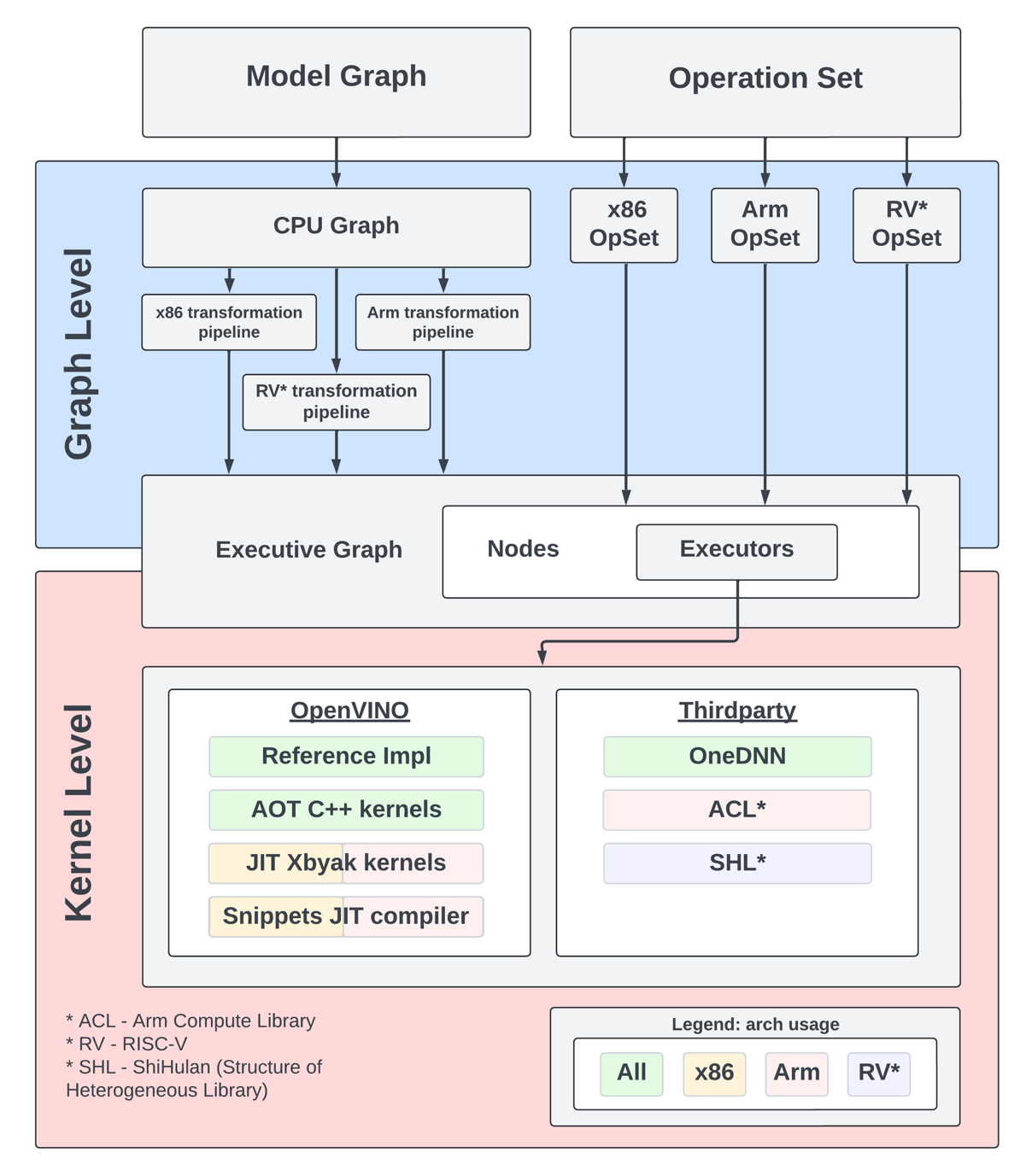
The OpenVINO CPU plugin architecture is divided into two main parts: the graph level and the execution kernel level, as shown in Diagram 1. The graph level involves optimizing the base graph of the AI model and converting it into an internal representation, using information about the processor architecture, computation specifics, algorithm characteristics, and more. The kernel level contains a set of computational kernels packaged into executors for various platforms. This set of computational kernels is divided into two main groups: kernels implemented directly within OpenVINO, and kernels utilized from third-party libraries. These groups help to select the optimal solutions for all supported architectures.
It is important to highlight that OpenVINO includes a special optimization layer called graph transformations. The main goal of this layer is to optimize the computation of the model graph on the processor, as well as to determine the order of processing and execution of graph nodes (or to eliminate some nodes from computations). Additionally, this layer has two significant aspects. The wide set of general transformations helps the plugin adjust to new architectures and keeps the computation graph well-suited for each specific type, like x86 or ARM. Balancing between general and specific optimizations, this approach is a crucial part of processing the model graph before execution by the kernels.
Generic Approaches for Device-Specific Optimizations in the CPU Plugin:
The CPU plugin incorporates three primary approaches to enable efficient, device-specific optimizations. These approaches are fully adopted for ARM architecture:
- Compiler Approach (Snippets)
- Integration ofOpenVINO Graph Compiler(known as Snippets)
The CPU plugin integrates Snippets to optimize performance by identifying and reusing common patterns within the execution graph. This approach enhances computational efficiency and ensures adaptability across different tasks.
- Integration ofOpenVINO Graph Compiler(known as Snippets)
- OpenVINO internal kernels (JIT + AOT):
- JIT (Xbyak): The CPU plugin employs JIT-compiled kernels using Xbyak to dynamically generate optimized code at runtime.
- AOT (Optimal Reference Implementation): Precompiled kernels developed within the OpenVINO framework provide efficient, reusable solutions for computational tasks.
- Third-Party Libraries
The CPU plugin leverages third-party libraries to access pre-optimized kernels for ARM:- Direct Use ofARM Compute Library(ACL) Kernels:
By directly using kernels from the ARM Compute Library (ACL), the plugin exploits the library’s inherent advantages for ARM-based computations. - Accessing ACL Kernels viaOneDNN:
The plugin accesses and optimizes ACL kernels through OneDNN, ensuring comprehensive coverage of ACL’s capabilities. - Accessing Other ARM-Optimized Kernels via OneDNN:
Beyond ACL, the plugin supports additional ARM-optimized kernels available through OneDNN, enabling broader model compatibility.
- Direct Use ofARM Compute Library(ACL) Kernels:
It is also important to address the topic of parallelism. In the context of OpenVINO, there are two levels of parallelism: graph-level parallelism and kernel-level parallelism. This approach enables optimal distribution of the processor load and maximizes the use of computational resources. Due to its complexity, a custom interface for parallelism is necessary, which incorporates particular libraries and standards for parallel computing. For ARM architecture support in OpenVINO, the current parallelism approach employs the OpenMP standard or the OneTBB library. OpenVINO uses OneTBB as the default threading backend, offering scalability and efficient task scheduling for high-performance applications. For users who prefer OpenMP, OpenVINO can be recompiled from source to enable OpenMP support. This flexibility allows developers to tailor threading options to specific project needs.For users who prefer OpenMP, OpenVINO can be recompiled from source to enable OpenMP support. This flexibility allows developers to tailor threading options to specific project needs.
Additionally, it is useful to briefly explain the role of external third-party libraries in OpenVINO.
To gain a deeper understanding of the context, we will discuss key libraries such as ARM Compute Library and OneDNN. These libraries are crucial for enhancing performance and reducing memory consumption in the OpenVINO CPU plugin for ARM architecture.
Arm Compute Library
The Arm Compute Library is an open-source collection of software optimized for Cortex-A CPUs, Neoverse systems, and Mali GPUs. It offers superior performance compared to other open-source alternatives and rapidly integrates new Arm technologies like SVE2. Key features include over 100 machine learning functions for CPU and GPU, support for multiple convolution algorithms (GEMM, Winograd, FFT, Direct), and various data types (FP32, FP16, int8, uint8, BFloat16). The library provides micro-architecture optimizations for key ML primitives, highly configurable build options for lightweight binaries, and advanced techniques such as Kernel Fusion, Fast math, and texture utilization. Additionally, it supports device and workload-specific tuning with OpenCL tuner and GEMM-optimized heuristics.
OneDNN Library
Intel® oneAPI Deep Neural Network Library (oneDNN) provides highly optimized implementations for deep learning operations across CPUs, GPUs, and other hardware. Its unified API improves performance for frameworks such as OpenVINO, Intel AI Tools, PyTorch*, and TensorFlow*, streamlining development and deployment processes by eliminating the need for target-specific code.
This library is fundamental to OpenVINO as it is crucial for optimizing neural network inference on Intel processors. It has drawn interest for supporting various computational architectures, made possible by the developer community and the accessibility of its source code. For instance, the ARM Compute Library is used for ARM architectures, along with JIT kernels integrated by Fujitsu. This variety enables achieving optimal performance on ARM architectures.
OpenVINO Distribution
The OpenVINO™ Runtime distribution for ARM devices provides various easy installation options. You can install OpenVINO via an archive file, use Python's PyPI, Conda Forge, Homebrew for macOS, Microsoft's vcpkg package manager, or Conan Package Manager. Detailed instructions are provided for each method to help you through the setup.
OpenVINO Notebooks
OpenVINO notebooks provide tutorials and step-by-step guides for various deep learning tasks. They cover a range of topics from setup process to model optimization and deployment. The notebooks are useful for learners at all levels, providing clear explanations and examples to help you learn OpenVINO.
The demos below demonstrate several notebooks running locally on Apple Mac M1 Pro Laptop and Apple Mac M2 Studio with OpenVINO™ 2025.0 release.
The Phi-3 Vision model is used for multimodal tasks, combining text and image processing. It can generate image descriptions, answer questions based on visual content, extract and analyze text from images, classify objects and scenes, and assist in content moderation.
https://drive.google.com/file/d/1-deK-heXq9B-iu4kAIO3ty8mDxLE3cnx/view?usp=sharing
Stable Diffusion 3 is a next-gen diffusion model using MMDiT, offering superior image quality, typography, and prompt adherence with improved efficiency.
https://drive.google.com/file/d/1HDB_d8sTkvqAstoq39QzufCF3rvYYjjJ/view?usp=sharing
Yolo-v11 object detection example
YOLOv11 is a fast and efficient real-time object detection model with improved accuracy and optimized architecture. It supports tasks like detection, segmentation, and classification while being adaptable to various platforms.
https://drive.google.com/file/d/1ISlBEAQWpyiEvFo6aRDBlQcfnf0l-V3R/view?usp=sharing
Collaborating with the Open-source Community
Good First Issue tasks
Developers eager to help improve OpenVINO can start by tackling "good first issue" tickets for ARM devices, which are a helpful way to enhance OpenVINO's performance on ARM architectures.
Contributing to the development of the OpenVINO plugin for ARM devices involves optimizing performance, aligning with ARM's features, and tackling platform-specific challenges. The open-source community is actively working on the plugin, taking on advanced tasks like implementation of highly optimized JIT kernels.
Google Summer of Code
Last year, our team joined the Google Summer of Code with a project aimed at boosting the performance of Generative AI (GenAI) on ARM devices using the OpenVINO toolkit.
The project focused on decreasing latency, accelerating model compilation, and reducing memory consumption. It entailed creating a benchmarking system and using advanced optimization methods for ARM architectures in the OpenVINO ecosystem. This work was important for OpenVINO's growth as an open-source framework.
Conclusion
In summary, using the OpenVINO CPU plugin on ARM devices can significantly improve computational efficiency and accelerate inference tasks. Its optimization techniques and compatibility with ARM architectures help developers make the most of ARM-based platforms for diverse AI applications. As ARM devices become more common in different industries, OpenVINO toolkit stands out as a powerful way to get fast AI results with lower latency and power consumption. Additionally, the teamwork between Intel and the ARM community is driving new developments in AI deployment for desktops and servers.
OpenVINO deploying DeepSeek-R1 Model Server (OVMS) on Bare metal Windows AIPC
Authors: Kunda Xu, Sapala, Rafal A
DeepSeek-R1 is an open-source reasoning model developed by DeepSeek to address tasks requiring logical inference, mathematical problem-solving, and real-time decision-making. With DeepSeek-R1,you can follow its logic, making it easier to understand and, if necessary, challenge its output. This capability gives reasoning models an edge in fields where outcomes need to be explainable, like research or complex decision-making.
Distillation in AI creates smaller, more efficient models from larger ones, preserving much of their reasoning power while reducing computational demands. DeepSeek applied this technique to create a suite of distilled models from R1, using Qwen and Llama architectures. That allows us to try DeepSeek-R1 capability locally on usual laptops (AIPC).
In this tutorial, we consider deploy deepseek-ai/DeepSeek-R1-Distill-Qwen-7B as a model server on Intel AIPC or AI work station with Windows OS to perform request generation tasks.
Requirements:
- Windows11
- VC_redist : Microsoft Visual C++ Redistributable
- Intel iGPU or ARC GPU: Intel® Arc™ & Iris® Xe Graphics - Windows*
- OpenVINO >=2025.0 : https://github.com/openvinotoolkit/openvino/releases/tag/2025.0.0
- OVMS >=2025.0 : https://github.com/openvinotoolkit/model_server/releases/tag/v2025.0
QuickStart Guide
Step 1. Install python dependencies for the conversion script:
Step 2. Run optimum-cli to download and quantize the model:
If your network access to HuggingFace is unstable, you can try to use a proxy image to pull the model.
Step 3. Deploying Model Server (OVMS) on Bare metal
Download and unpack model server archive for Windows:
Run setupvars script to set required environment variables
Step 4. DeepSeek-R1 model server deploy
Bare metal Host deploy. Required: deploying ovms on Bera metal.
OpenVINO + OVMS can also use Docker contain deploying. Required: Docker engine installed
When using docker as a deployment method, you need to consider whether the hardware performance of the machine is sufficient, because docker contain will also generate additional memory overhead.
For example, when deploying on a laptop or AIPC, due to the limited memory resources, it is more reasonable to use bare metal deployment method
Step 5. Check readiness Wait for the model to load.
You can check the status with a simple command
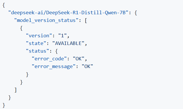
Step 6. Run model server generation
Create a file called request.json ,
and copy the following content into it
You will get the output like the following.
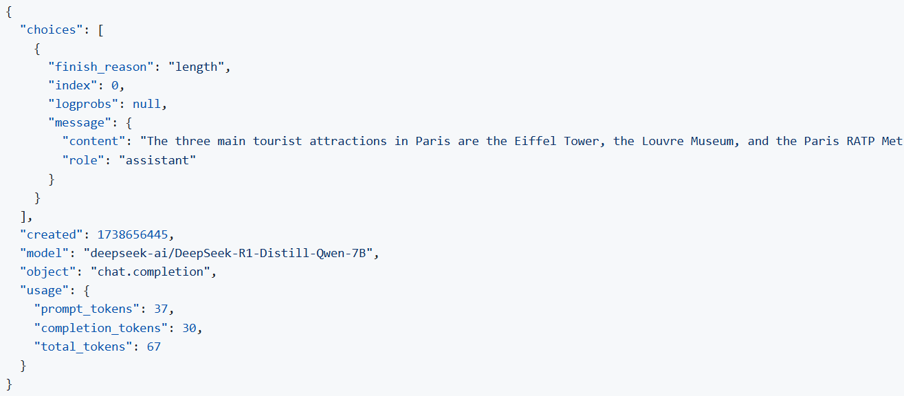
Note: If you want to get the response chunks streamed back as they are generated change stream parameter in the request to true
DeepSeek Janus-Pro Model Enabling with OpenVINO
1. Introduction
Janus is a unified multimodal understanding and generation model developed by DeepSeek. Janus proposed decoupling visual encoding to alleviate the conflict between multimodal understanding and generation tasks. Janus-Pro further scales up the Janus model to larger model size (deepseek-ai/Janus-Pro-1B & deepseek-ai/Janus-Pro-7B) with optimized training strategy and training data, achieving significant advancements in both multimodal understanding and text-to-image tasks.
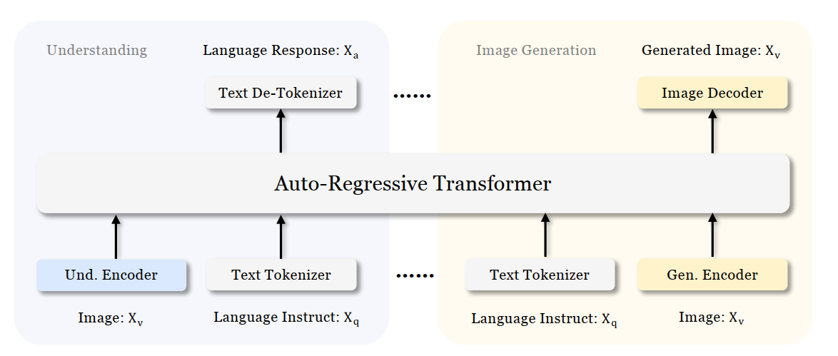
Figure 1 shows the architecture of Janus-Pro, which decouples visual encoding for multimodal understanding and visual generation. “Und. Encoder” and “Gen. Encoder” are abbreviations for “Understanding Encoder” and “Generation Encoder”. For the multimodal understanding task, SigLIP vision encoder used to extract high-dimensional semantic features from the image, while for the vision generation task, VQ tokenizer used to map images to discrete IDs. Both the understanding adaptor and the generation adaptor are two-layer MLPs to map the embeddings to the input space of LLM.
In this blog, we will introduce how to deploy Janus-Pro model with OpenVINOTM runtime on the intel platform.
2. Janus-Pro Pytorch Model to OpenVINOTM Model Conversion
2.1. Setup Python Environment
2.2 Download Janus Pytorch model (Optional)
2.3. Convert Pytorch Model to OpenVINOTM INT4 Model
The converted OpenVINO will be saved in Janus-Pro-1B-OV directory for deployment.
3. Janus-Pro Inference with OpenVINOTM Demo
In this section, we provide several examples to show Janus-Pro for multimodal understanding and vision generation tasks.
3.1. Multimodal Understanding Task – Image Caption with OpenVINOTM
Prompt: Describe image in details
Input image:

Generated Output:
3.2. Multimodal Understanding Task – Equation Description with OpenVINOTM
Prompt: Generate the latex code of this formula
Input Image:
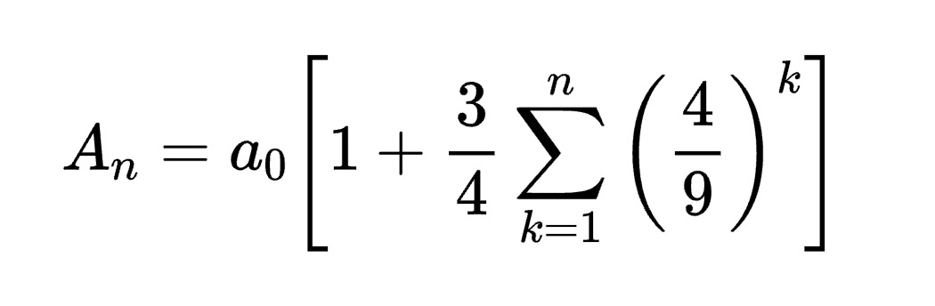
Generated Output:
3.3. Multimodal Understanding Task – Code Generation with OpenVINOTM
Prompt: Generate the matplotlib pyplot code for this plot
Input Image:
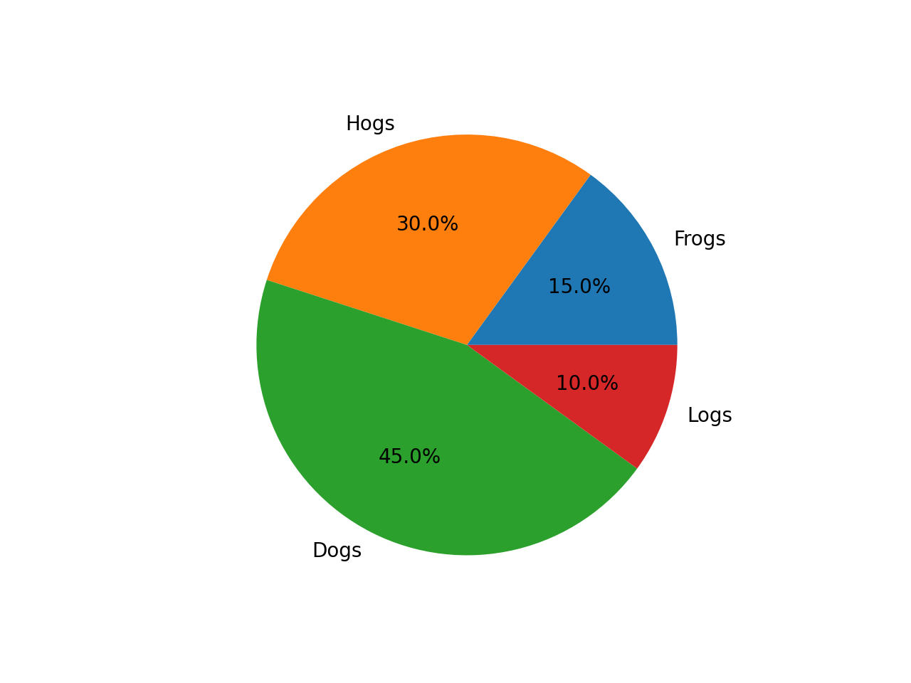
Generated Output:
3.4. Vision Generation Task with OpenVINOTM
Input Prompt: A cute and adorable baby fox with big brown eyes, autumn leaves in the background enchanting, immortal, fluffy, shiny mane, Petals, fairyism, unreal engine 5 and Octane Render, highly detailed, photorealistic, cinematic, natural colors.
Generated image:


4. Performance Evaluation & Memory Usage Analysis
We also provide benchmark scripts to evaluate Janus-Pro model performance and memory usage with OpenVINOTM inference, you may specify model name and device for your target platform.
4.1. Benchmark Janus-Pro for Multimodal Understanding Task with OpenVINOTM
Here are some arguments for benchmark script for Multimodal Understanding Task:
--model_id: specify the Janus OpenVINOTM model directory
--prompt: specify input prompt for multimodal understanding task
--image_path: specify input image for multimodal understanding task
--niter: specify number of test iteration, default is 5
--device: specify which device to run inference
--max_new_tokens: specify max number of generated tokens
By default, the benchmark script will run 5 round multimodal understanding tasks on target device, then report pipeline initialization time, average first token latency (including preprocessing), 2nd+ token throughput and max RSS memory usage.
4.2. Benchmark Janus-Pro for Text-to-Image Task with OpenVINOTM
Here are some arguments for benchmark scripts for Text-to-Image Task
--model_id: specify the Janus OpenVINO TM model directory
--prompt: specify input prompt for text-to-image generation task
--niter: specify number of test iteration
--device: specify which device to run inference
By default, the benchmark script will run 5 round image generation tasks on target device, then report the pipeline initialization time, average image generation latency and max RSS memory usage.
5. Conclusion
In this blog, we introduced how to enable Janus-Pro model with OpenVINOTM runtime, then we demonstrated the Janus-Pro capability for various multimodal understanding and image generation tasks. In the end, we provide python script for performance & memory usage evaluation for both multimodal understanding and image generation task on target platform.